Visualizing weather data in Google Earth
Note: This article describes the assessment work for the course Scientific Visualization lectured at Grenoble Institute of Technology (winter semester 2015/2016).
Introduction
The goal of this project was to visualize data from Meteo France in Google Earth using several methods presented in the course. Meteo France provides publicly available weather data such as temperatures or atmospheric pressures at several locations. The work consists of the following four main steps:
- read and import the scattered data (longitude, latitude, temperature, pressure, and wind velocity)
- interpolate the scattered data in order to evaluate data at arbitrary positions, using the Shepard’s method and the Hardy multiquadrics
- calculate colormap images and isocontours from the interpolated data
- export the colormap images and the isocontours in a KML (Keyhole Markup Language) file in order to visualize the data in Google Earth
In several next sections, you can find the results of this task and also a detailed description of individual steps of the implementation which lead to the final visualization.
Solution
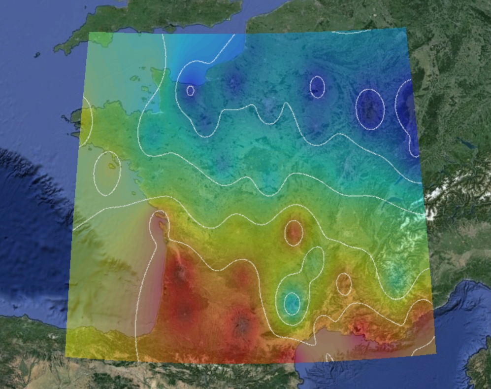
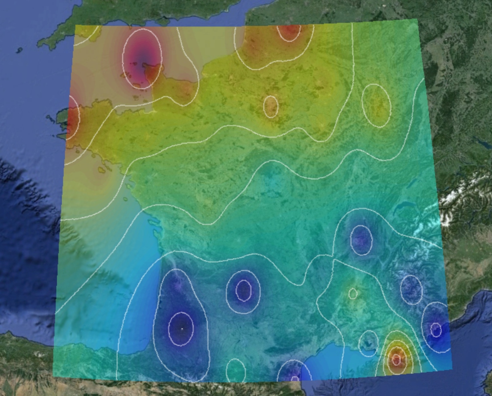
I have carried out this project using C++ programming language. First, I am attaching several test visualizations that have been exported to Google Earth in order to verify the correctness of the code output. You can find the result in Figure 1.
The data processing pipeline which goes from the initial data reading to the final visualization is hardcoded in function run_visualization that is shown below:
1
2
3
4
5
6
7
8
9
10
11
12
void run_visualization(std::string input_file) {
  weather_data quantity;
  quantity.load_data(input_file);
  quantity.create_grid({1025, 1025});
  quantity.shepard_interpolation(2.0);
  /*quantity.hardy_interpolation(2.0);*/
  quantity.compute_colormap(jet);
  quantity.compute_isolines(6);
  quantity.export_colormap();
  quantity.export_isolines();
  return;
}
By default, the size of grid is set to 1025 nodes in both directions, which leads to the size of generated colormap 1024 x 1024. Then the Shepard’s interpolation with parameter p = 2 is performed. For the colormap, the predefined color table jet with 64 colors is used. After that, 6 isolines are computed, and both, colormap and isolines, are exported to the KML file. One can change the arguments, uncomment one of the methods for interpolation, but the order of the data processing pipeline has to be kept as is.
For the code compilation, one can use attached bash script compile.sh which executes prepared Makefile. Due to the usage of features introduced in C++14, the minimum required version of GCC compiler is 4.8. Compiled application takes the filename of the input data as an argument. Both, the application and the input file, have to be located in the same directory.
Implementation details
Tip: The source code of this work can be found in this GitHub repository.
The main idea how to deal with several steps of the implementation was to make a single class for the data processing, which includes data structures for scattered and uniform data as well as all methods beginning with reading of the input data and ending with the required visualization. One can find the listings of this class below, individual methods and data structures will be described later.
1
2
3
4
5
6
7
8
9
10
11
12
13
14
15
16
17
18
19
class weather_data {
public:
  weather_data();
  void load_data(std::string input_file);
  void create_grid(std::array<unsigned int, 2> size);
  weather_data& shepard_interpolation(double p);
  weather_data& hardy_interpolation(double R);
  weather_data& compute_colormap(std::vector<std::array<int, 4>> color_table);
  weather_data& compute_isolines(unsigned int n);
  void export_colormap();
  void export_isolines();
  ~weather_data();
private:
  std::string name;
  uniform_data uniform;
  scattered_data scattered;
  std::vector<unsigned char> colormap;
  std::vector<isoline> isolines;
};
The main advantage of this approach is simpler and faster way to access the data during the interpolation of scattered data to the uniform grid. The drawback is obviously inability to use the code for solving other similar problems as well as more difficult development of the code extensions.
Reading input data
The first step is to gather and parse the data. Meteo France provides publicly available data including atmospheric parameters measured at several France meteorological stations in the CSV (Comma-Separated Values) file format. For the purposes of the project, we are interested in temperature, atmospheric pressure and wind velocity. Since all the data undergo the same process before the final visualization, the data are loaded from separate CSV files, which have to contain three columns. The first two are dedicated for latitude and longitude of the site and the last one for the value of the measured parameter.
Scattered data are parsed into the following data structure:
1
2
3
4
5
typedef struct {
  unsigned int size;
  std::array<double, 4> boundary;
  std::vector<std::array<double, 3>> values;
} scattered_data;
The size value stands for the number of rows in the input file (number of the stations), the boundary stores minimum and maximum coordinates, and the array of three vectors values is dedicated for the data itself.
The responsibility for the data parsing takes the following method:
1
2
3
4
5
6
7
8
9
10
11
12
13
14
15
16
17
18
19
20
21
22
23
24
25
26
27
28
29
30
31
32
33
34
35
36
37
38
39
void weather_data::load_data(std::string filename) {
  std::ifstream input_file;
  std::string line;
  std::cout << "loading scattered data: " << filename << std::endl;
  this->name = filename.substr(0, filename.find_last_of("."));
  input_file.open(filename);
  if(input_file.fail()) {
    std::cerr << "error: cannot read input file" << std::endl;
    return;
  }
  this->scattered.size = 0;
  while(std::getline(input_file, line)) {
    ++this->scattered.size;
  }
  input_file.clear();
  input_file.seekg(0, std::ios::beg);
  this->scattered.values.resize(this->scattered.size);
  if(input_file.is_open()) {
    for(std::size_t i = 0; i < this->scattered.size; ++i) {
      for(std::size_t j = 0; j < 3; ++j) {
        input_file >> this->scattered.values[i][j];
        input_file.get();
      }
    }
  }
  double min_x = this->scattered.values[0][0];
  double max_x = this->scattered.values[0][0];
  double min_y = this->scattered.values[0][1];
  double max_y = this->scattered.values[0][1];
  for(std::size_t i = 0; i < this->scattered.size; ++i) {
    min_x = std::min(min_x, this->scattered.values[i][0]);
    max_x = std::max(max_x, this->scattered.values[i][0]);
    min_y = std::min(min_y, this->scattered.values[i][1]);
    max_y = std::max(max_y, this->scattered.values[i][1]);
  }
  this->scattered.boundary = {min_x, max_x, min_y, max_y};
  std::cout << "scattered data loaded successfully" << std::endl;
  return;
}
This method reads and imports the data from a given file, finds the boundaries and stores the name of the file.
Creating uniform grid
Since the input data are loaded, we need to create a two-dimensional uniform grid to be able to perform interpolation. Similarly as before, we need a data structure for uniform data:
1
2
3
4
5
6
7
typedef struct {
  std::array<unsigned int, 2> size;
  std::array<double, 2> spacing;
  std::array<double, 4> boundary;
  std::vector<std::vector<cell>> cells;
  std::vector<std::vector<node>> nodes;
} uniform_data;
This data structure contains the size of the grid, which is now a pair of integers (number of nodes in x and y directions), spacing between two nodes in both directions, minimum and maximum coordinates, the matrix of cells and the matrix of nodes.
The matrices of cells and nodes use special datastructures. The first datastructure is cell:
1
2
3
4
5
6
7
8
9
10
11
12
13
14
15
16
17
18
class cell {
  friend class weather_data;
public:
  cell() = default;
  segment top_bottom();
  segment top_left();
  segment top_right();
  segment bottom_left();
  segment bottom_right();
  segment left_right();
  cell& compute_average();
  ~cell() = default;
private:
  int id;
  double average;
  std::array<int, 4> RGBA;
  std::array<node*, 4> nodes;
};
This class contains ID, four pointers to the nodes assigned to the cell, average of the node values and RGBA color space, which will take a value determined by the average (in order to calculate the colormap). In addition, this class includes the method for computing the average value of nodes assigned to the cell as well as several methods for selecting a segment of this cell in order to compute isocontours. The segment data structure contains only coordinates of the starting and ending points:
1
2
3
4
5
6
7
8
9
10
class segment {
  friend class cell;
  friend class weather_data;
public:
  segment() = default;
  ~segment() = default;
private:
  std::array<double, 2> start;
  std::array<double, 2> end;
};
The second data type is used to describe nodes. This class is much simpler than the cell class, it contains only ID and three floating point numbers: latitude, longitude and the value of measured parameter:
1
2
3
4
5
6
7
8
9
10
class node {
  friend class cell;
  friend class weather_data;
public:
  node() = default;
  ~node() = default;
private:
  int id;
  std::array<double, 3> values;
};
The second step in the data processing pipeline is to create a two-dimensional uniform grid. For this purpose, there is a method in the main class:
1
2
3
4
5
6
7
8
9
10
11
12
13
14
15
16
17
18
19
20
21
22
23
24
25
26
27
28
29
30
31
32
33
34
35
36
37
38
39
40
41
42
43
44
45
46
47
void weather_data::create_grid(std::array<unsigned int, 2> size) {
  if(!size[0] || !size[1]) {
    std::cerr << "error: cannot create grid" << std::endl;
    return;
  }
  std::cout << "creating uniform grid of size: " << size[0] << " x " << size[1] << std::endl;
  this->uniform.size = {
    size[0],
    size[1]
  };
  this->uniform.boundary = this->scattered.boundary;
  this->uniform.spacing = {
    (this->uniform.boundary[1] - this->uniform.boundary[0]) / this->uniform.size[0],
    (this->uniform.boundary[3] - this->uniform.boundary[2]) / this->uniform.size[1]
  };
  this->uniform.nodes.resize(this->uniform.size[1]);
  for(std::size_t i = 0; i < this->uniform.size[1]; ++i) {
    this->uniform.nodes[i].resize(this->uniform.size[0]);
  }
  for(std::size_t i = 0; i < this->uniform.size[1]; ++i) {
    for(std::size_t j = 0; j < this->uniform.size[0]; ++j) {
      this->uniform.nodes[i][j].id = this->uniform.size[0] * i + j;
      this->uniform.nodes[i][j].values[0] = this->uniform.boundary[0] + j * this->uniform.spacing[0];
      this->uniform.nodes[i][j].values[1] = this->uniform.boundary[2] + i * this->uniform.spacing[1];
      this->uniform.nodes[i][j].values[2] = 0.0;
    }
  }
  this->uniform.cells.resize(this->uniform.size[1] - 1);
  for(std::size_t i = 0; i < this->uniform.size[1] - 1; ++i) {
    this->uniform.cells[i].resize(this->uniform.size[0] - 1);
  }
  for(std::size_t i = 0; i < this->uniform.size[1] - 1; ++i) {
    for(std::size_t j = 0; j < this->uniform.size[0] - 1; ++j) {
      this->uniform.cells[i][j].id = (this->uniform.size[0] - 1) * i + j;
      this->uniform.cells[i][j].average = 0.0;
      this->uniform.cells[i][j].RGBA = {0, 0, 0, 255};
      this->uniform.cells[i][j].nodes = {
        &this->uniform.nodes[i][j],
        &this->uniform.nodes[i][j + 1],
        &this->uniform.nodes[i + 1][j + 1],
        &this->uniform.nodes[i + 1][j],
      };
    }
  }
  std::cout << "uniform grid created successfully" << std::endl;
  return;
}
This method takes the size of the grid in both directions as an argument. The grid size significantly affects the quality and the computational time of the interpolation as well as the resolution of the computed colormap and the smoothness of the isocontours. The location of the grid is done automatically in accordance with the boundaries of the scattered data. This method also initializes the cells and nodes.
Performing interpolation
The crucial step is the interpolation of scattered data in order to evaluate measured parameters at the grid points. In accordance with the project specifications, two following methods have been used:
Shepard’s method
The principle of finding an interpolated value of scattered data $ f_{i} = f\left( \vec{x}_{i} \right) $ for $ i \in \left\lbrace 1, \ldots, N \right\rbrace $ at a given point $ \vec{x} $ using Shepard’s method, is based on constructing an interpolating function
\[\small{F \left( \vec{x} \right) = \sum_{i = 1}^{N} \omega_{i} \left( \vec{x} \right) f_{i}},\]where the weighting function $ \omega_{i} \left( \vec{x} \right) $ is defined by Shepard as follows [1],
\[\small{\omega_{i} \left( \vec{x} \right) = \frac{1}{\mathrm{d} \left( \vec{x}, \: \vec{x}_{i}\right) ^{p}} \cdot \frac{1}{\sum \limits_{j = 1}^{N} \frac{1}{\mathrm{d} \left( \vec{x}, \: \vec{x}_{j}\right) ^{p}}}},\] \[\small{\mathrm{d}\left( \vec{x}, \: \vec{x}_{i} \right) = \lVert \vec{x} - \vec{x}_{i} \rVert}\]and $ p $ is a positive real number, called the power parameter.
The implementation of this method is attached below. In the first step, the weighting function $ \omega_{i} \left( \vec{x} \right) $ is calculated for each grid point. Afterwards, the measured parameter is evaluated there.
1
2
3
4
5
6
7
8
9
10
11
12
13
14
15
16
17
18
19
20
21
22
23
24
25
weather_data& weather_data::shepard_interpolation(double p) {
  std::cout << "performing interpolation using the sheppard method with parameter p = " << p << std::endl;
  std::vector<std::vector<double>> w;
  w.resize(this->uniform.size[1]);
  for(std::size_t i = 0; i < this->uniform.size[1]; ++i) {
    w[i].resize(this->uniform.size[0]);
  }
  for(std::size_t i = 0; i < this->uniform.size[1]; ++i) {
    for(std::size_t j = 0; j < this->uniform.size[0]; ++j) {
      w[i][j] = 0.0;
      this->uniform.nodes[i][j].values[2] = 0.0;
      for(std::size_t k = 0; k < this->scattered.size; ++k) {
        w[i][j] += 1.0 / pow(sqrt(pow(this->uniform.nodes[i][j].values[0] - this->scattered.values[k][0], 2)
        + pow(this->uniform.nodes[i][j].values[1] - this->scattered.values[k][1], 2)), p);
      }
      for(std::size_t k = 0; k < this->scattered.size; ++k) {
        this->uniform.nodes[i][j].values[2] += (1.0 / pow(sqrt(pow(this->uniform.nodes[i][j].values[0]
        - this->scattered.values[k][0], 2) + pow(this->uniform.nodes[i][j].values[1]
        - this->scattered.values[k][1], 2)), p)) * (1.0 / w[i][j]) * this->scattered.values[k][2];
      }
    }
  }
  std::cout << "scattered data successfully interpolated to uniform grid" << std::endl;
  return (*this);
}
Hardy multiquadrics
The second method which has been implemented is called Hardy multiquadrics. Now, we are looking for the interpolating function in the following form [2],
\(\small{F\left( \vec{x} \right) = \sum_{i = 1}^{N} \alpha_{i} h_{i} \left( \vec{x} \right)},\)
where $ \alpha_{i} $ are unknown coefficients and
\(\small{h_{i} \left( \vec{x} \right) = \sqrt{R + \mathrm{d} \left( \vec{x}, \: \vec{x}_{i} \right)^{2} }}.\)
The input argument R is a nonzero shape parameter. The coefficients $ \alpha_{i} $ are calculated by solving the system of equations given by the conditions
\(\small{F\left( \vec{x}_{i} \right) = f_{i}}.\)
It was proven by [3] that for distinct data, this system of equations is always solvable.
The implementation of the Hardy’s method has been carried out as follows:
1
2
3
4
5
6
7
8
9
10
11
12
13
14
15
16
17
18
19
20
21
22
23
24
25
26
27
28
weather_data& weather_data::hardy_interpolation(double R) {
  std::cout << "performing interpolation using the hardy multiquadrics with parameter R = " << R << std::endl;
  Eigen::MatrixXd b(this->scattered.size, this->scattered.size);
  Eigen::VectorXd alpha(this->scattered.size);
  Eigen::VectorXd f(this->scattered.size);
  for(std::size_t k = 0; k < this->scattered.size; ++k) {
    f(k) = this->scattered.values[k][2];
    for(std::size_t l = 0; l < this->scattered.size; ++l) {
      b(k, l) = sqrt(R + pow(this->scattered.values[k][0] - this->scattered.values[l][0], 2)
      + pow(this->scattered.values[k][1] - this->scattered.values[l][1], 2));
    }
  }
  alpha = b.lu().solve(f);
  std::vector<double> h;
  h.resize(this->scattered.size);
  for(std::size_t i = 0; i < this->uniform.size[1]; ++i) {
    for(std::size_t j = 0; j < this->uniform.size[0]; ++j) {
      this->uniform.nodes[i][j].values[2] = 0.0;
      for(std::size_t k = 0; k < this->scattered.size; ++k) {
        h[k] = sqrt(R + pow(this->uniform.nodes[i][j].values[0] - this->scattered.values[k][0], 2)
        + pow(this->uniform.nodes[i][j].values[1] - this->scattered.values[k][1], 2));
        this->uniform.nodes[i][j].values[2] += alpha(k) * h[k];
      }
    }
  }
  std::cout << "scattered data successfully interpolated to uniform grid" << std::endl;
  return (*this);
}
The system of linear equations is solved using LU decomposition from the Eigen C++ library. Then the function $ h_{i} \left( \vec{x} \right) $ is calculated at each grid point and the measured parameter is evaluated there.
Calculating colormaps
Since we have interpolated values of measured parameter at each grid point, one is able to compute a colormap. The idea is to calculate an average value of the four nodes assigned to each cell. Then the maximum and minimum of average values are determined and the interval formed by these two numbers is divided into several parts corresponding to the number of colors in the color table. Afterwards, each cell will get the RGB value from the color table according to its average value. The implementation has been done as follows:
1
2
3
4
5
6
7
8
9
10
11
12
13
14
15
16
17
18
19
20
21
22
23
24
25
26
27
28
29
30
weather_data& weather_data::compute_colormap(std::vector<std::array<int, 4>> color_table) {
  std::cout << "computing colormap.. " << std::endl;
  double max = 0.0;
  double min = std::numeric_limits<double>::infinity();
  for(std::size_t i = 0; i < this->uniform.size[1] - 1; ++i) {
    for(std::size_t j = 0; j < this->uniform.size[0] - 1; ++j) {
      this->uniform.cells[i][j].compute_average();
      max = std::max(max, this->uniform.cells[i][j].average);
      min = std::min(min, this->uniform.cells[i][j].average);
    }
  }
  unsigned int n = color_table.size();
  double span = (max - min) / n;
  std::cout << "number of colors: " << n << std::endl;
  this->colormap.resize((this->uniform.size[0] - 1) * (this->uniform.size[1] - 1) * 4);
  for(std::size_t i = 0; i < this->uniform.size[1] - 1; ++i) {
    for(std::size_t j = 0; j < this->uniform.size[0] - 1; ++j) {
      for(std::size_t k = 0; k < n; ++k) {
        if(this->uniform.cells[i][j].average <= min + (k + 1) * span && this->uniform.cells[i][j].average >= min + k * span) {
          this->uniform.cells[i][j].RGBA = color_table[k];
        }
      }
      for(std::size_t k = 0; k < 4; ++k) {
        this->colormap[4 * ((this->uniform.size[1] - i - 2) * (this->uniform.size[0] - 1) + j) + k] = this->uniform.cells[i][j].RGBA[k];
      }
    }
  }
  std::cout << "colormap created successfully" << std::endl;
  return (*this);
}
Calculating isocontours
Similarly as before, the method for computing isocontours takes a number of isocontours as an argument. Then the maximum and minimum of values assigned to grid points are calculated, and the interval, which these two numbers form, is divided by the number of isocontours we want to calculate. The isocontours are computed in accordance with these thresholds using so called marching squares algorithm. My implementation of the marching squares algorithm is shown below:
1
2
3
4
5
6
7
8
9
10
11
12
13
14
15
16
17
18
19
20
21
22
23
24
25
26
27
28
29
30
31
32
33
34
35
36
37
38
39
40
41
42
43
44
45
46
47
48
49
50
51
52
53
54
55
56
57
58
59
60
61
62
63
64
65
66
67
68
69
70
71
72
73
74
75
76
77
78
weather_data& weather_data::compute_isolines(unsigned int n) {
  std::cout << "computing isolines.. " << std::endl;
  this->isolines.resize(n);
  std::cout << "number of isolines: " << n << std::endl;
  std::vector<double> thresholds;
  double max = 0.0;
  double min = std::numeric_limits<double>::infinity();
  for(std::size_t i = 0; i < this->uniform.size[1]; ++i) {
    for(std::size_t j = 0; j < this->uniform.size[0]; ++j) {
      max = std::max(max, this->uniform.nodes[i][j].values[2]);
      min = std::min(min, this->uniform.nodes[i][j].values[2]);
    }
  }
  double span = (max - min) / (n + 1);
  for(std::size_t i = 0; i < n; i++) {
    thresholds.push_back(min + i * span);
  }
  unsigned int bits;
  for(size_t l = 0; l < this->isolines.size(); ++l) {
    this->isolines[l].value = thresholds[l];
    for(std::size_t i = 0; i < this->uniform.size[1] - 1; ++i) {
      for(std::size_t j = 0; j < this->uniform.size[0] - 1; ++j) {
        bits = 0;
        for(std::size_t k = 0; k < 4; ++k) {
          if(this->uniform.cells[i][j].nodes[k]->values[2] > this->isolines[l].value) {
            bits |= 1 << (3 - k);
          }
        }
        switch(bits) {
          case 0: case 15:
            break;
          case 1: case 14:
            this->isolines[l].segments.push_back(this->uniform.cells[i][j].bottom_left());
            break;
          case 2: case 13:
            this->isolines[l].segments.push_back(this->uniform.cells[i][j].bottom_right());
            break;
          case 3: case 12:
            this->isolines[l].segments.push_back(this->uniform.cells[i][j].left_right());
            break;
          case 4: case 11:
            this->isolines[l].segments.push_back(this->uniform.cells[i][j].top_right());
            break;
          case 6: case 9:
            this->isolines[l].segments.push_back(this->uniform.cells[i][j].top_bottom());
            break;
          case 7: case 8:
            this->isolines[l].segments.push_back(this->uniform.cells[i][j].top_left());
            break;
          case 5:
            if(this->uniform.cells[i][j].average > this->isolines[l].value) {
              this->isolines[l].segments.push_back(this->uniform.cells[i][j].top_left());
              this->isolines[l].segments.push_back(this->uniform.cells[i][j].bottom_right());
            } else {
              this->isolines[l].segments.push_back(this->uniform.cells[i][j].top_right());
              this->isolines[l].segments.push_back(this->uniform.cells[i][j].bottom_left());
            }
            break;
          case 10:
            if(this->uniform.cells[i][j].average > this->isolines[l].value) {
              this->isolines[l].segments.push_back(this->uniform.cells[i][j].top_right());
              this->isolines[l].segments.push_back(this->uniform.cells[i][j].bottom_left());
            }
            else {
              this->isolines[l].segments.push_back(this->uniform.cells[i][j].top_left());
              this->isolines[l].segments.push_back(this->uniform.cells[i][j].bottom_right());
            }
            break;
          default:
            std::cerr << "error: unknown error" << std::endl;
            break;
        }
      }
    }
  }
  std::cout << "isolines computed successfully" << std::endl;
  return (*this);
}
Exporting data
In order to visualize the calculated data in Google Earth, it is necessary to export them in the KML file format. Regarding the colormap, first we need to export the generated image in PNG format. For this reason, the LodePNG C++ libriary has been used. Then we need to generate a KML file with the specified path to the colormap image and the coordinates, where this image should appear. These coordinates are determined by boundaries that we computed before. For the isocontours, we need to export separate line segments determined by its starting and ending points. These lines we have computed before as segments. Altogether, they create a whole isoline.
There exists a KML library written in C++ called libkml, but it is deprecated. Therefore, I decided to write my own methods for exporting the data into a KML file. One can find it in the source code.
References
[1] Shepard, D., “A two-dimensional interpolation function for irregularly-spaced data”, Proceedings of the 1968 ACM National Conference, pp. 517 - 524.
[2] Hardy, R., “Multiquadric equations of topography and other irregular surfaces”, Journal of Geophysical Research 76, pp. 1905 - 1915 (1971).
[3] Micchelli, C., “Interpolation of scattered data: Distance matrices and conditionally positive definite functions”, Constructive Approximation 2, pp. 11 – 22 (1986).